Cyber insurance and Data - Part II: Coalition's Florida admitted model


This blog post was co-written with Mitch Peterson, Pricing Actuary at Swiss Re Corporate Solutions
The second part of our Cyber insurance and Data series describes how we (quite literally) integrated technology variables, traditional rating factors, and mathematical methods from the Casualty Actuary Society to file one of the first admitted cyber products in the state of Florida. You can read the first part of the series here.
This post breaks down our approach into two steps. First, we develop a process to construct a dataset useful for modeling cyber risk. Second, we review the math behind pricing insurance contracts, and apply that to the losses contained within the dataset.
Data
At Coalition, data collection and processing is a key focus of our business. Fortunately for us, data is also a crucial ingredient of a successful justifiable rating plan, so we were able to approach this model filing as a natural extension of the work we do on a daily basis.
In data collection, there are two components to consider: variables and observations.
Variables
While almost all insurers will collect the revenue and industry of an applicant, we run a large-scale in-house data collection system. This collection system provides us a dataset with many variables per observation, like this (hypothetical) example set of two companies:
Linked Entry ID: 1mGcX5zqQPUHVK09j20deJ
We love variables because the more variables we can collect, the better we can separate high risk and low risk applicants, prioritize loss-reducing interventions, and effectively price to risk.
To show how additional variables can increase the power of our models, let's start with a single variable — the number of personally identifiable information records stored by a company.
We can regress this on the severity, in dollars, of losses suffered during a claim to notice this positive (though messy) trend:
If you hover your mouse over the trend line, you can observe details of the line of best fit, including an <img class="inline" src="https://chart.googleapis.com/chart?cht=tx&chl=R^2"> value of around .33.
<img class="inline" src="https://chart.googleapis.com/chart?cht=tx&chl=R^2">, pronounced "R squared" and also known as the coefficient of determination, is a classical measure of model fit, with higher values indicating a better relationship between the outcome value and variables of interest
Now, If we can expand our dataset from one variable to two (let's say, are_ssns_encrypted: [True, False]), we can greatly increase the accuracy of the model to predict loss severity. The following graph is the exact same data points, but breaking out losses with the new variable:
By moving your cursor over the lines of best fit, you can observe significantly higher values of <img class="inline" src="https://chart.googleapis.com/chart?cht=tx&chl=R^2"> in this new stratified analysis.
Observations
What's the downside of many variables? With traditional statistical techniques, having many more variables than observations can lead to issues of statistical significance and an increased chance of falsely concluding a variable is important. For example, the aforementioned <img class="inline" src="https://chart.googleapis.com/chart?cht=tx&chl=R^2"> is not as useful in the presence of many explanatory variables
1. We use widely-accepted techniques of feature penalization, like AIC, to remove features that do add sufficient explanatory value
2. We follow qualitative expert judgement from our cybersecurity teams to remove variables where we have doubts about the relationship between the variable and true risk of the insured.
3. We augment our policyholder data with additional observations obtained from third-party sources, increasing the size of our ultimate data set
To illustrate the gain of additional observations, see how increasing the number of observations improves the fit of the previous example.
Data, meet math!
Now that we have our dataset, we follow the modeling techniques laid out in the Casualty Actuary Society's Generalized Linear Models for Insurance Rating. A key output of the model training process is the statistical distribution f(x), the estimated distribution of the severity of a claim, which varies based on x, the available information about the insured.
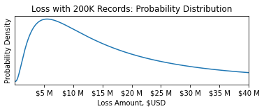
At this point, it's important to understand the difference between a predicted value and the distribution of that value, called the prediction interval. In the linear fit example of loss severity on record count, the predicted loss severity value for 200,000 records and unencrypted SSNs would be $20MM. For the purpose of pricing an insurance contract, however, we need to model the statistical distribution of that loss amount, and it is critical that the resulting probabilities are accurate.
For example, even if we are confident the average loss is $20MM, we need to know the probability of a loss being larger than $50MM. Thankfully, generalized linear models incorporate modeling this distribution as part of the fitting process.
Finally, to use these tools to quantify the risk of an insurance contract, we must consider the deductible ("d") and limit ("l") of the insuring agreement. For small losses under the deductible, the covered loss amount is zero. After losses surpass the deductible, the insuring agreement covers all losses until it has paid out the full limit. At this point, the total loss amount is equal to the sum of the deductible and the limit.
This means we can estimate the average insurable loss as the sum of two integrals over the severity distribution f(x) . The first integral covers the situations where the loss is above the retention but below paying out full limit, and the second integral covers losses where the full limit will be paid out:
<img src="https://chart.googleapis.com/chart?cht=tx&chl=average%20loss(x,d,l)=\int_{d}^{d%2Bl}{(t-d)%20f(t,x)%20dt}%20%2B%20l%20\int_{d%2Bl}^{\infty}%20{f(t,x)%20dt}">
(Astute readers may notice that the second integral is simply the limit multiplied by the probability of a full limit loss)
We can combine all aspects of this blog post into an interactive tool that breaks down the integral into its constituent parts and prices the insurance policy:
If you've made it this far, consider joining us! We are looking for people who are excited to tackle large problems and join us in our mission to solve cyber risk. If that sounds like you, please check out our job postings.
Related blog posts
Control Cyber Risk from the Inside Out
Coalition Control™ integrates with cloud providers Microsoft 365, Google Workspace, and AWS to allow customers to manage digital risks in a single platform.

Cyber Incident Reporting: Important Questions to Ask for Essential Business Planning
Cyber incident reporting obligations can be complex. Businesses must consider how they will meet the requirements before an incident to expedite the process.